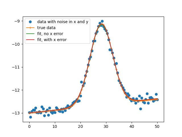
Fitting data with uncertainties in x and y

This examples shows a general way of fitting a model to y(x) data which has uncertainties in both y and x.

For more in-depth discussion, see

https://dx.doi.org/10.1021/acs.analchem.0c02178

### not including uncertainty in x:
[[Fit Statistics]]
    # fitting method   = leastsq
    # function evals   = 62
    # data points      = 101
    # variables        = 5
    chi-square         = 344.228513
    reduced chi-square = 3.58571368
    Akaike info crit   = 133.844705
    Bayesian info crit = 146.920308
[[Variables]]
    amp:     38.7909094 +/- 0.54820333 (1.41%) (init = 50)
    cen:     28.1858429 +/- 0.05334483 (0.19%) (init = 25)
    sig:     4.44210577 +/- 0.05938737 (1.34%) (init = 10)
    slope:   0.01260816 +/- 8.1762e-04 (6.48%) (init = 0.0001)
    offset: -13.0004948 +/- 0.02386032 (0.18%) (init = -5)
[[Correlations]] (unreported correlations are < 0.100)
    C(slope, offset) = -0.7603
    C(amp, sig)      = +0.7056
    C(amp, offset)   = -0.2735
    C(cen, slope)    = -0.2460
    C(amp, slope)    = -0.2115
    C(sig, offset)   = -0.1924
    C(cen, offset)   = +0.1870
    C(sig, slope)    = -0.1495
None
### including uncertainty in x:
[[Fit Statistics]]
    # fitting method   = leastsq
    # function evals   = 43
    # data points      = 101
    # variables        = 5
    chi-square         = 223.406586
    reduced chi-square = 2.32715193
    Akaike info crit   = 90.1811577
    Bayesian info crit = 103.256760
[[Variables]]
    amp:     39.2776438 +/- 0.94011531 (2.39%) (init = 50)
    cen:     28.1731192 +/- 0.12633327 (0.45%) (init = 25)
    sig:     4.44581423 +/- 0.09870523 (2.22%) (init = 10)
    slope:   0.01252275 +/- 6.7955e-04 (5.43%) (init = 0.0001)
    offset: -13.0005237 +/- 0.01980939 (0.15%) (init = -5)
[[Correlations]] (unreported correlations are < 0.100)
    C(amp, sig)      = +0.8188
    C(slope, offset) = -0.7475
    C(amp, offset)   = -0.2037
    C(cen, slope)    = -0.1715
    C(sig, offset)   = -0.1655
    C(amp, slope)    = -0.1630
    C(cen, offset)   = +0.1381
    C(sig, slope)    = -0.1359
None
[0.01438036 0.52896805 1.04666251 1.58348091]

import matplotlib.pyplot as plt
import numpy as np

from lmfit import Minimizer, Parameters, report_fit
from lmfit.lineshapes import gaussian

# create data to be fitted
np.random.seed(17)
xtrue = np.linspace(0, 50, 101)
xstep = xtrue[1] - xtrue[0]
amp, cen, sig, offset, slope = 39, 28.2, 4.4, -13, 0.012

ytrue = (gaussian(xtrue, amplitude=amp, center=cen, sigma=sig)
         + offset + slope * xtrue)

ydat = ytrue + np.random.normal(size=xtrue.size, scale=0.1)

# we add errors to x after y has been created, as if there is
# an ideal y(x) and we have noise in both x and y.
# we force the uncertainty away from 'normal', forcing
# it to be smaller than the step size.
xerr = np.random.normal(size=xtrue.size, scale=0.1*xstep)
max_xerr = 0.8*xstep
xerr[np.where(xerr > max_xerr)] = max_xerr
xerr[np.where(xerr < -max_xerr)] = -max_xerr
xdat = xtrue + xerr

# now we assert that we know the uncertaintits in y and x
#   we'll pick values that are reesonable but not exactly
#   what we used to make the noise
yerr = 0.06
xerr = xstep


def peak_model(params, x):
    """Model a peak with a linear background."""
    amp = params['amp'].value
    cen = params['cen'].value
    sig = params['sig'].value
    offset = params['offset'].value
    slope = params['slope'].value
    return offset + slope * x + gaussian(x, amplitude=amp, center=cen, sigma=sig)


# objective without xerr
def objective_no_xerr(params, x, y, yerr):
    model = peak_model(params, x)
    return (model - y) / abs(yerr)


# objective with xerr
def objective_with_xerr(params, x, y, yerr, xerr):
    model = peak_model(params, x)
    dmodel_dx = np.gradient(model) / np.gradient(x)
    dmodel = np.sqrt(yerr**2 + (xerr*dmodel_dx)**2)
    return (model - y) / dmodel


# create a set of Parameters
params = Parameters()
params.add('amp', value=50, min=0)
params.add('cen', value=25)
params.add('sig', value=10)
params.add('slope', value=1.e-4)
params.add('offset', value=-5)

# first fit without xerr
mini1 = Minimizer(objective_no_xerr, params, fcn_args=(xdat, ydat, yerr))
result1 = mini1.minimize()
bestfit1 = peak_model(result1.params, xdat)


mini2 = Minimizer(objective_with_xerr, params, fcn_args=(xdat, ydat, yerr, xerr))
result2 = mini2.minimize()

bestfit2 = peak_model(result2.params, xdat)


print("### not including uncertainty in x:")
print(report_fit(result1))
print("### including uncertainty in x:")
print(report_fit(result2))

print(xdat[:4])

plt.plot(xdat, ydat, 'o', label='data with noise in x and y')
plt.plot(xtrue, ytrue, '-+', label='true data')
plt.plot(xdat, bestfit1, label='fit, no x error')
plt.plot(xdat, bestfit2, label='fit, with x error')
plt.legend()
plt.show()

# # <end examples/doc_uncertainties_in_x_and_y.py>