Complex Resonator Model

This notebook shows how to fit the parameters of a complex resonator, using lmfit.Model and defining a custom Model class.

Following Khalil et al. (https://arxiv.org/abs/1108.3117), we can model the forward transmission of a microwave resonator with total quality factor \(Q\), coupling quality factor \(Q_e\), and resonant frequency \(f_0\) using:

\[S_{21}(f) = 1 - \frac{Q Q_e^{-1}}{1+2jQ(f-f_0)/f_0}\]

\(S_{21}\) is thus a complex function of a real frequency.

By allowing \(Q_e\) to be complex, this model can take into account mismatches in the input and output transmission impedances.

import matplotlib.pyplot as plt
import numpy as np

import lmfit

Since scipy.optimize and lmfit require real parameters, we represent \(Q_e\) as Q_e_real + 1j*Q_e_imag.

def linear_resonator(f, f_0, Q, Q_e_real, Q_e_imag):
    Q_e = Q_e_real + 1j*Q_e_imag
    return 1 - (Q * Q_e**-1 / (1 + 2j * Q * (f - f_0) / f_0))

The standard practice of defining a lmfit model is as follows:

class ResonatorModel(lmfit.model.Model):
    __doc__ = "resonator model" + lmfit.models.COMMON_INIT_DOC

    def __init__(self, *args, **kwargs):
        # pass in the defining equation so the user doesn't have to later
        super().__init__(linear_resonator, *args, **kwargs)

        self.set_param_hint('Q', min=0)  # enforce Q is positive

    def guess(self, data, f=None, **kwargs):
        verbose = kwargs.pop('verbose', None)
        if f is None:
            return
        argmin_s21 = np.abs(data).argmin()
        fmin = f.min()
        fmax = f.max()
        f_0_guess = f[argmin_s21]  # guess that the resonance is the lowest point
        Q_min = 0.1 * (f_0_guess/(fmax-fmin))  # assume the user isn't trying to fit just a small part of a resonance curve
        delta_f = np.diff(f)  # assume f is sorted
        min_delta_f = delta_f[delta_f > 0].min()
        Q_max = f_0_guess/min_delta_f  # assume data actually samples the resonance reasonably
        Q_guess = np.sqrt(Q_min*Q_max)  # geometric mean, why not?
        Q_e_real_guess = Q_guess/(1-np.abs(data[argmin_s21]))
        if verbose:
            print(f"fmin={fmin}, fmax={fmax}, f_0_guess={f_0_guess}")
            print(f"Qmin={Q_min}, Q_max={Q_max}, Q_guess={Q_guess}, Q_e_real_guess={Q_e_real_guess}")
        params = self.make_params(Q=Q_guess, Q_e_real=Q_e_real_guess, Q_e_imag=0, f_0=f_0_guess)
        params[f'{self.prefix}Q'].set(min=Q_min, max=Q_max)
        params[f'{self.prefix}f_0'].set(min=fmin, max=fmax)
        return lmfit.models.update_param_vals(params, self.prefix, **kwargs)

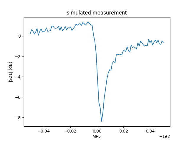
Now let’s use the model to generate some fake data:

resonator = ResonatorModel()
true_params = resonator.make_params(f_0=100, Q=10000, Q_e_real=9000, Q_e_imag=-9000)

f = np.linspace(99.95, 100.05, 100)
true_s21 = resonator.eval(params=true_params, f=f)
noise_scale = 0.02
np.random.seed(123)
measured_s21 = true_s21 + noise_scale*(np.random.randn(100) + 1j*np.random.randn(100))

plt.plot(f, 20*np.log10(np.abs(measured_s21)))
plt.ylabel('|S21| (dB)')
plt.xlabel('MHz')
plt.title('simulated measurement')

Try out the guess method we added:

guess = resonator.guess(measured_s21, f=f, verbose=True)

fmin=99.95, fmax=100.05, f_0_guess=100.00353535353536
Qmin=100.00353535354105, Q_max=99003.50000055433, Q_guess=3146.537781821432, Q_e_real_guess=5082.2474265369565

And now fit the data using the guess-ed values as a starting point:

result = resonator.fit(measured_s21, params=guess, f=f, verbose=True)

print(result.fit_report() + '\n')
result.params.pretty_print()

[[Model]]
    Model(linear_resonator)
[[Fit Statistics]]
    # fitting method   = leastsq
    # function evals   = 41
    # data points      = 200
    # variables        = 4
    chi-square         = 0.08533642
    reduced chi-square = 4.3539e-04
    Akaike info crit   = -1543.89425
    Bayesian info crit = -1530.70099
    R-squared          = (-12528141463701.6+2276419599932.454j)
[[Variables]]
    f_0:       100.000096 +/- 7.0308e-05 (0.00%) (init = 100.0035)
    Q:         10059.4972 +/- 142.294636 (1.41%) (init = 3146.538)
    Q_e_real:  9180.62017 +/- 133.777681 (1.46%) (init = 5082.247)
    Q_e_imag: -9137.03667 +/- 133.769692 (1.46%) (init = 0)
[[Correlations]] (unreported correlations are < 0.100)
    C(Q, Q_e_real)   = +0.5175
    C(f_0, Q_e_imag) = +0.5175
    C(f_0, Q_e_real) = +0.5151
    C(Q, Q_e_imag)   = -0.5150

Name         Value      Min      Max   Stderr     Vary     Expr Brute_Step
Q         1.006e+04      100  9.9e+04    142.3     True     None     None
Q_e_imag     -9137     -inf      inf    133.8     True     None     None
Q_e_real      9181     -inf      inf    133.8     True     None     None
f_0            100    99.95      100 7.031e-05     True     None     None

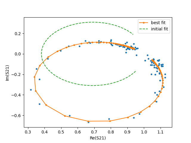
Now we’ll make some plots of the data and fit. Define a convenience function for plotting complex quantities:

def plot_ri(data, *args, **kwargs):
    plt.plot(data.real, data.imag, *args, **kwargs)


fit_s21 = resonator.eval(params=result.params, f=f)
guess_s21 = resonator.eval(params=guess, f=f)

plt.figure()
plot_ri(measured_s21, '.')
plot_ri(fit_s21, '.-', label='best fit')
plot_ri(guess_s21, '--', label='initial fit')
plt.legend()
plt.xlabel('Re(S21)')
plt.ylabel('Im(S21)')

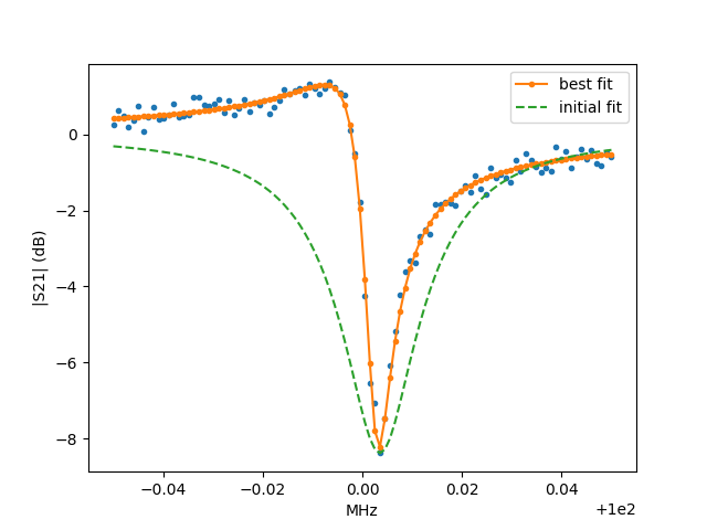
plt.figure()
plt.plot(f, 20*np.log10(np.abs(measured_s21)), '.')
plt.plot(f, 20*np.log10(np.abs(fit_s21)), '.-', label='best fit')
plt.plot(f, 20*np.log10(np.abs(guess_s21)), '--', label='initial fit')
plt.legend()
plt.ylabel('|S21| (dB)')
plt.xlabel('MHz')

• 
•