Calculation of confidence intervals¶

The lmfit confidence module allows you to explicitly calculate confidence intervals for variable parameters. For most models, it is not necessary since the estimation of the standard error from the estimated covariance matrix is normally quite good.

But for some models, the sum of two exponentials for example, the approximation begins to fail. For this case, lmfit has the function conf_interval() to calculate confidence intervals directly. This is substantially slower than using the errors estimated from the covariance matrix, but the results are more robust.

Please note that conf_interval() is not suited to work with fit results obtained by emcee.

Method used for calculating confidence intervals¶

The F-test is used to compare our null model, which is the best fit we have found, with an alternate model, where one of the parameters is fixed to a specific value. The value is changed until the difference between \(\chi^2_0\) and \(\chi^2_{f}\) can’t be explained by the loss of a degree of freedom within a certain confidence.

\[F(P_{fix},N-P) = \left(\frac{\chi^2_f}{\chi^2_{0}}-1\right)\frac{N-P}{P_{fix}}\]

N is the number of data points and P the number of parameters of the null model. \(P_{fix}\) is the number of fixed parameters (or to be more clear, the difference of number of parameters between our null model and the alternate model).

Adding a log-likelihood method is under consideration.

A basic example¶

First we create an example problem:

import numpy as np

import lmfit

x = np.linspace(0.3, 10, 100)
np.random.seed(0)
y = 1/(0.1*x) + 2 + 0.1*np.random.randn(x.size)
pars = lmfit.Parameters()
pars.add_many(('a', 0.1), ('b', 1))


def residual(p):
    return 1/(p['a']*x) + p['b'] - y

before we can generate the confidence intervals, we have to run a fit, so that the automated estimate of the standard errors can be used as a starting point:

mini = lmfit.Minimizer(residual, pars)
result = mini.minimize()

print(lmfit.fit_report(result.params))

[[Variables]]
    a:  0.09943896 +/- 1.9322e-04 (0.19%) (init = 0.1)
    b:  1.98476942 +/- 0.01222678 (0.62%) (init = 1)
[[Correlations]] (unreported correlations are < 0.100)
    C(a, b) = +0.6008

Now it is just a simple function call to calculate the confidence intervals:

ci = lmfit.conf_interval(mini, result)
lmfit.printfuncs.report_ci(ci)

      99.73%    95.45%    68.27%    _BEST_    68.27%    95.45%    99.73%
 a:  -0.00059  -0.00039  -0.00019   0.09944  +0.00019  +0.00039  +0.00060
 b:  -0.03764  -0.02477  -0.01229   1.98477  +0.01229  +0.02477  +0.03764

This shows the best-fit values for the parameters in the _BEST_ column, and parameter values that are at the varying confidence levels given by steps in \(\sigma\). As we can see, the estimated error is almost the same, and the uncertainties are well behaved: Going from 1-\(\sigma\) (68% confidence) to 3-\(\sigma\) (99.7% confidence) uncertainties is fairly linear. It can also be seen that the errors are fairly symmetric around the best fit value. For this problem, it is not necessary to calculate confidence intervals, and the estimates of the uncertainties from the covariance matrix are sufficient.

Working without standard error estimates¶

Sometimes the estimation of the standard errors from the covariance matrix fails, especially if values are near given bounds. Hence, to find the confidence intervals in these cases, it is necessary to set the errors by hand. Note that the standard error is only used to find an upper limit for each value, hence the exact value is not important.

To set the step-size to 10% of the initial value we loop through all parameters and set it manually:

for p in result.params:
    result.params[p].stderr = abs(result.params[p].value * 0.1)

Calculating and visualizing maps of \(\chi^2\)¶

The estimated values for the \(1-\sigma\) standard error calculated by default for each fit include the effects of correlation between pairs of variables, but assumes the uncertainties are symmetric. While it doesn’t exactly say what the values of the \(n-\sigma\) uncertainties would be, the implication is that the \(n-\sigma\) error is simply \(n^2\sigma\).

The conf_interval() function described above improves on these automatically (and quickly) calculated uncertainies by explicitly finding \(n-\sigma\) confidence levels in both directions – it does not assume that the uncertainties are symmetric. This function also takes into account the correlations between pairs of variables, but it does not convey this information very well.

For even further exploration of the confidence levels of parameter values, it can be useful to calculate maps of \(\chi^2\) values for pairs of variables around their best fit values and visualize these as contour plots. Typically, pairs of variables will have elliptical contours of constant \(n-\sigma\) level, with highly-correlated pairs of variables having high ratios of major and minor axes.

The conf_interval2d() can calculate 2-d arrays or maps of either probability or \(\delta \chi^2 = \chi^2 - \chi_{\mathrm{best}}^2\) for any pair of variables. Visualizing these can help better understand the nature of the uncertainties and correlations between parameters. To illustrate this, we’ll start with an example fit to data that we deliberately add components not accounted for in the model, and with slightly non-Gaussian noise – a constructed but “real-world” example:

# <examples/doc_confidence_chi2_maps.py>
import matplotlib.pyplot as plt
import numpy as np

from lmfit import conf_interval, conf_interval2d, report_ci
from lmfit.lineshapes import gaussian
from lmfit.models import GaussianModel, LinearModel

sigma_levels = [1, 2, 3]

rng = np.random.default_rng(seed=102)

#########################
# set up data -- deliberately adding imperfections and
# a small amount of non-Gaussian noise
npts = 501
x = np.linspace(1, 100, num=npts)
noise = rng.normal(scale=0.3, size=npts) + 0.2*rng.f(3, 9, size=npts)
y = (gaussian(x, amplitude=83, center=47., sigma=5.)
     + 0.02*x + 4 + 0.25*np.cos((x-20)/8.0) + noise)

mod = GaussianModel() + LinearModel()
params = mod.make_params(amplitude=100, center=50, sigma=5,
                         slope=0, intecept=2)
out = mod.fit(y, params, x=x)
print(out.fit_report())

#########################
# run conf_intervale, print report
sigma_levels = [1, 2, 3]
ci = conf_interval(out, out, sigmas=sigma_levels)

print("## Confidence Report:")
report_ci(ci)

[[Model]]
    (Model(gaussian) + Model(linear))
[[Fit Statistics]]
    # fitting method   = leastsq
    # function evals   = 31
    # data points      = 501
    # variables        = 5
    chi-square         = 103.861381
    reduced chi-square = 0.20939794
    Akaike info crit   = -778.348033
    Bayesian info crit = -757.265003
    R-squared          = 0.93782756
[[Variables]]
    amplitude:  78.8171374 +/- 1.21910939 (1.55%) (init = 100)
    center:     47.0751649 +/- 0.07576660 (0.16%) (init = 50)
    sigma:      4.93298753 +/- 0.07984021 (1.62%) (init = 5)
    slope:      0.01839006 +/- 7.1957e-04 (3.91%) (init = 0)
    intercept:  4.39234411 +/- 0.04420227 (1.01%) (init = 0)
    fwhm:       11.6162977 +/- 0.18800933 (1.62%) == '2.3548200*sigma'
    height:     6.37412722 +/- 0.08603873 (1.35%) == '0.3989423*amplitude/max(1e-15, sigma)'
[[Correlations]] (unreported correlations are < 0.100)
    C(slope, intercept)     = -0.8421
    C(amplitude, sigma)     = +0.6371
    C(amplitude, intercept) = -0.3373
    C(sigma, intercept)     = -0.2149
    C(center, slope)        = -0.1026

## Confidence Report:
              99.73%    95.45%    68.27%    _BEST_    68.27%    95.45%    99.73%
 amplitude:  -3.62610  -2.41983  -1.21237  78.81714  +1.22111  +2.45479  +3.70515
 center   :  -0.22849  -0.15214  -0.07584  47.07516  +0.07587  +0.15225  +0.22873
 sigma    :  -0.23335  -0.15640  -0.07870   4.93299  +0.08000  +0.16158  +0.24509
 slope    :  -0.00217  -0.00144  -0.00072   0.01839  +0.00072  +0.00144  +0.00217
 intercept:  -0.13326  -0.08860  -0.04423   4.39234  +0.04421  +0.08854  +0.13312

The reports show that we obtained a pretty good fit, and that the automated estimates of the uncertainties are actually pretty good – agreeing to the second decimal place. But we also see that some of the uncertainties do become noticeably asymmetric at high \(n-\sigma\) levels.

We’ll plot this data and fit, and then further explore these uncertainties using conf_interval2d(). Please note that conf_interval2d() shows the confidence intervals obtained considering the standard errors, not those obtained by ‘conf_interval(out, out, sigmas=sigma_levels)’.

#########################
# plot initial fit
colors = ('#2030b0', '#b02030', '#207070')
fig, axes = plt.subplots(2, 3, figsize=(15, 9.5))

axes[0, 0].plot(x, y, 'o', markersize=3, label='data', color=colors[0])
axes[0, 0].plot(x, out.best_fit, label='fit', color=colors[1])
axes[0, 0].set_xlabel('x')
axes[0, 0].set_ylabel('y')
axes[0, 0].legend()

aix, aiy = 0, 0
nsamples = 50
explicitly_calculate_sigma = True

for pairs in (('sigma', 'amplitude'), ('intercept', 'amplitude'),
              ('slope', 'intercept'), ('slope', 'center'), ('sigma', 'center')):

    xpar, ypar = pairs
    if explicitly_calculate_sigma:
        print(f"Generating chi-square map for {pairs}")
        c_x, c_y, chi2_mat = conf_interval2d(out, out, xpar, ypar,
                                             nsamples, nsamples, nsigma=3.5,
                                             chi2_out=True)
        # explicitly calculate sigma matrix: sigma increases chi_square
        # from  chi_square_best
        # to    chi_square + sigma**2 * reduced_chi_square
        # so:   sigma = sqrt((chi2-chi2_best)/ reduced_chi_square)
        chi2_min = chi2_mat.min()
        sigma_mat = np.sqrt((chi2_mat-chi2_min)/out.redchi)
    else:
        print(f"Generating sigma map for {pairs}")
        # or, you could just calculate the matrix of probabilities as:
        c_x, c_y, sigma_mat = conf_interval2d(out, out, xpar, ypar,
                                              nsamples, nsamples, nsigma=3.5)

    aix += 1
    if aix == 2:
        aix = 0
        aiy += 1
    ax = axes[aix, aiy]

    cnt = ax.contour(c_x, c_y, sigma_mat, levels=sigma_levels, colors=colors,
                     linestyles='-')
    ax.clabel(cnt, inline=True, fmt=r"$\sigma=%.0f$", fontsize=13)

    # draw boxes for estimated uncertaties:
    #  dotted :  scaled stderr from initial fit
    #  dashed :  values found from conf_interval()
    xv = out.params[xpar].value
    xs = out.params[xpar].stderr
    yv = out.params[ypar].value
    ys = out.params[ypar].stderr

    cix = ci[xpar]
    ciy = ci[ypar]
    nc = len(sigma_levels)
    for i in sigma_levels:
        # dotted line: scaled stderr
        ax.plot((xv-i*xs, xv+i*xs, xv+i*xs, xv-i*xs, xv-i*xs),
                (yv-i*ys, yv-i*ys, yv+i*ys, yv+i*ys, yv-i*ys),
                linestyle='dotted', color=colors[i-1])

        # dashed line: refined uncertainties from conf_interval
        xsp, xsm = cix[nc+i][1], cix[nc-i][1]
        ysp, ysm = ciy[nc+i][1], ciy[nc-i][1]
        ax.plot((xsm, xsp, xsp, xsm, xsm), (ysm, ysm, ysp, ysp, ysm),
                linestyle='dashed', color=colors[i-1])

    ax.set_xlabel(xpar)
    ax.set_ylabel(ypar)
    ax.grid(True, color='#d0d0d0')
plt.show()
# <end examples/doc_confidence_chi2_maps.py>

Generating chi-square map for ('sigma', 'amplitude')

Generating chi-square map for ('intercept', 'amplitude')

Generating chi-square map for ('slope', 'intercept')

Generating chi-square map for ('slope', 'center')

Generating chi-square map for ('sigma', 'center')

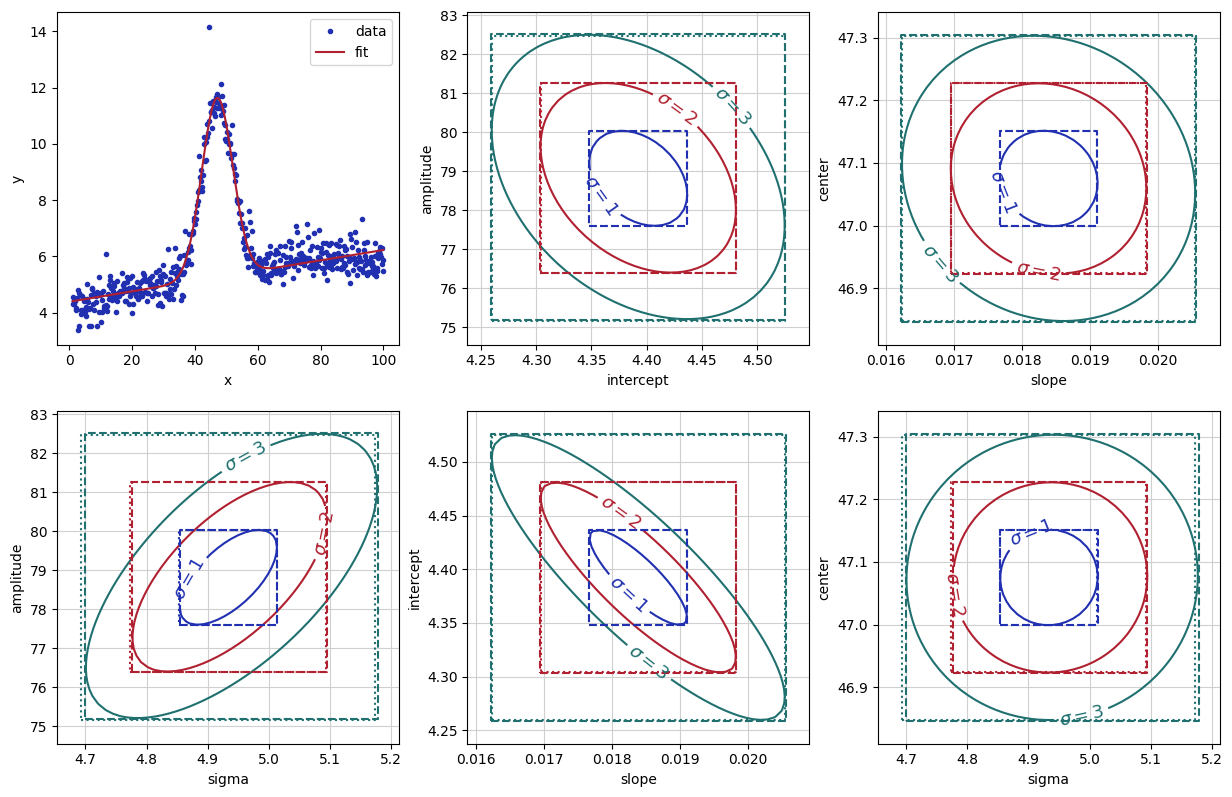
Here we made contours for the \(n-\sigma\) levels from the 2-D array of \(\chi^2\) by noting that the \(n-\sigma\) level will have \(\chi^2\) increased by \(n^2\chi_\nu^2\) where \(\chi_\nu^2\) is reduced chi-square.

The dotted boxes show both the scaled values of the standard errors from the initial fit, and the dashed boxes show the confidence levels from conf_interval(). You can see that the notion of increasing \(\chi^2\) by \(\chi_\nu^2\) works very well, and that there is a small asymmetry in the uncertainties for the amplitude and sigma parameters.

An advanced example for evaluating confidence intervals¶

Now we look at a problem where calculating the error from approximated covariance can lead to misleading result – the same double exponential problem shown in Minimizer.emcee() - calculating the posterior probability distribution of parameters. In fact such a problem is particularly hard for the Levenberg-Marquardt method, so we first estimate the results using the slower but robust Nelder-Mead method. We can then compare the uncertainties computed (if the numdifftools package is installed) with those estimated using Levenberg-Marquardt around the previously found solution. We can also compare to the results of using emcee.

# <examples/doc_confidence_advanced.py>
import matplotlib.pyplot as plt
import numpy as np

import lmfit

x = np.linspace(1, 10, 250)
np.random.seed(0)
y = 3.0*np.exp(-x/2) - 5.0*np.exp(-(x-0.1)/10.) + 0.1*np.random.randn(x.size)

p = lmfit.create_params(a1=4, a2=4, t1=3, t2=3)


def residual(p):
    return p['a1']*np.exp(-x/p['t1']) + p['a2']*np.exp(-(x-0.1)/p['t2']) - y


# create Minimizer
mini = lmfit.Minimizer(residual, p, nan_policy='propagate')

# first solve with Nelder-Mead algorithm
out1 = mini.minimize(method='Nelder')

# then solve with Levenberg-Marquardt using the
# Nelder-Mead solution as a starting point
out2 = mini.minimize(method='leastsq', params=out1.params)

lmfit.report_fit(out2.params, min_correl=0.5)

ci, trace = lmfit.conf_interval(mini, out2, sigmas=[1, 2], trace=True)
lmfit.printfuncs.report_ci(ci)

# plot data and best fit
plt.figure()
plt.plot(x, y)
plt.plot(x, residual(out2.params) + y, '-')
plt.show()

# plot confidence intervals (a1 vs t2 and a2 vs t2)
fig, axes = plt.subplots(1, 2, figsize=(12.8, 4.8))
cx, cy, grid = lmfit.conf_interval2d(mini, out2, 'a1', 't2', 30, 30)
ctp = axes[0].contourf(cx, cy, grid, np.linspace(0, 1, 11))
fig.colorbar(ctp, ax=axes[0])
axes[0].set_xlabel('a1')
axes[0].set_ylabel('t2')

cx, cy, grid = lmfit.conf_interval2d(mini, out2, 'a2', 't2', 30, 30)
ctp = axes[1].contourf(cx, cy, grid, np.linspace(0, 1, 11))
fig.colorbar(ctp, ax=axes[1])
axes[1].set_xlabel('a2')
axes[1].set_ylabel('t2')
plt.show()

# plot dependence between two parameters
fig, axes = plt.subplots(1, 2, figsize=(12.8, 4.8))
cx1, cy1, prob = trace['a1']['a1'], trace['a1']['t2'], trace['a1']['prob']
cx2, cy2, prob2 = trace['t2']['t2'], trace['t2']['a1'], trace['t2']['prob']

axes[0].scatter(cx1, cy1, c=prob, s=30)
axes[0].set_xlabel('a1')
axes[0].set_ylabel('t2')

axes[1].scatter(cx2, cy2, c=prob2, s=30)
axes[1].set_xlabel('t2')
axes[1].set_ylabel('a1')
plt.show()
# <end examples/doc_confidence_advanced.py>

which will report:

[[Variables]]
    a1:  2.98622095 +/- 0.14867027 (4.98%) (init = 2.986237)
    a2: -4.33526363 +/- 0.11527574 (2.66%) (init = -4.335256)
    t1:  1.30994276 +/- 0.13121215 (10.02%) (init = 1.309932)
    t2:  11.8240337 +/- 0.46316956 (3.92%) (init = 11.82408)
[[Correlations]] (unreported correlations are < 0.500)
    C(a2, t2) = +0.9871
    C(a2, t1) = -0.9246
    C(t1, t2) = -0.8805
    C(a1, t1) = -0.5988

       95.45%    68.27%    _BEST_    68.27%    95.45%
 a1:  -0.27285  -0.14165   2.98622  +0.16354  +0.36343
 a2:  -0.30440  -0.13219  -4.33526  +0.10689  +0.19684
 t1:  -0.23392  -0.12494   1.30994  +0.14660  +0.32369
 t2:  -1.01937  -0.48813  11.82403  +0.46045  +0.90439

Again we called conf_interval(), this time with tracing and only for 1- and 2-\(\sigma\). Comparing these two different estimates, we see that the estimate for a1 is reasonably well approximated from the covariance matrix, but the estimates for a2 and especially for t1, and t2 are very asymmetric and that going from 1 \(\sigma\) (68% confidence) to 2 \(\sigma\) (95% confidence) is not very predictable.

Plots of the confidence region are shown in the figures below for a1 and t2 (left), and a2 and t2 (right):

Neither of these plots is very much like an ellipse, which is implicitly assumed by the approach using the covariance matrix. The plots actually look quite a bit like those found with MCMC and shown in the “corner plot” in Minimizer.emcee() - calculating the posterior probability distribution of parameters. In fact, comparing the confidence interval results here with the results for the 1- and 2-\(\sigma\) error estimated with emcee, we can see that the agreement is pretty good and that the asymmetry in the parameter distributions are reflected well in the asymmetry of the uncertainties.

The trace returned as the optional second argument from conf_interval() contains a dictionary for each variable parameter. The values are dictionaries with arrays of values for each variable, and an array of corresponding probabilities for the corresponding cumulative variables. This can be used to show the dependence between two parameters:

fig, axes = plt.subplots(1, 2, figsize=(12.8, 4.8))
cx1, cy1, prob = trace['a1']['a1'], trace['a1']['t2'], trace['a1']['prob']
cx2, cy2, prob2 = trace['t2']['t2'], trace['t2']['a1'], trace['t2']['prob']

axes[0].scatter(cx1, cy1, c=prob, s=30)
axes[0].set_xlabel('a1')
axes[0].set_ylabel('t2')

axes[1].scatter(cx2, cy2, c=prob2, s=30)
axes[1].set_xlabel('t2')
axes[1].set_ylabel('a1')

plt.show()

which shows the trace of values:

As an alternative/complement to the confidence intervals, the Minimizer.emcee() method uses Markov Chain Monte Carlo to sample the posterior probability distribution. These distributions demonstrate the range of solutions that the data supports and we refer to Minimizer.emcee() - calculating the posterior probability distribution of parameters where this methodology was used on the same problem.

Credible intervals (the Bayesian equivalent of the frequentist confidence interval) can be obtained with this method. MCMC can be used for model selection, to determine outliers, to marginalize over nuisance parameters, etcetera. For example, you may have fractionally underestimated the uncertainties on a dataset. MCMC can be used to estimate the true level of uncertainty on each data point. A tutorial on the possibilities offered by MCMC can be found at [1].

Confidence Interval Functions¶

conf_interval(minimizer, result, p_names=None, sigmas=None, trace=False, maxiter=200, verbose=False, prob_func=None, min_rel_change=1e-05)¶

Calculate the confidence interval (CI) for parameters.

The parameter for which the CI is calculated will be varied, while the remaining parameters are re-optimized to minimize the chi-square. The resulting chi-square is used to calculate the probability with a given statistic (e.g., F-test). This function uses a 1d-rootfinder from SciPy to find the values resulting in the searched confidence region.

Parameters:

minimizer (Minimizer) – The minimizer to use, holding objective function.
result (MinimizerResult) – The result of running minimize().
p_names (list, optional) – Names of the parameters for which the CI is calculated. If None (default), the CI is calculated for every parameter.
sigmas (list, optional) – The sigma-levels to find (default is [1, 2, 3]). See Notes below.
trace (bool, optional) – Defaults to False; if True, each result of a probability calculation is saved along with the parameter. This can be used to plot so-called “profile traces”.
maxiter (int, optional) – Maximum of iteration to find an upper limit (default is 200).
verbose (bool, optional) – Print extra debugging information (default is False).
prob_func (None or callable, optional) – Function to calculate the probability from the optimized chi-square. Default is None and uses the built-in function f_compare (i.e., F-test).
min_rel_change (float, optional) – Minimum relative change in probability (default is 1e-5).

Returns:

output (dict) – A dictionary containing a list of (sigma, vals)-tuples for each parameter.
trace_dict (dict, optional) – Only if trace is True. Is a dictionary, the key is the parameter which was fixed. The values are again a dict with the names as keys, but with an additional key ‘prob’. Each contains an array of the corresponding values.

Table of Contents

Previous topic

Next topic