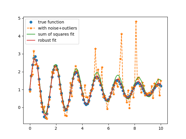
Fit Specifying Different Reduce Function

The reduce_fcn specifies how to convert a residual array to a scalar value for the scalar minimizers. The default value is None (i.e., “sum of squares of residual”) - alternatives are: negentropy, neglogcauchy, or a user-specified callable. For more information please refer to: https://lmfit.github.io/lmfit-py/fitting.html#using-the-minimizer-class

Here, we use as an example the Student’s t log-likelihood for robust fitting of data with outliers.

import matplotlib.pyplot as plt
import numpy as np

import lmfit


def resid(params, x, ydata):
    decay = params['decay'].value
    offset = params['offset'].value
    omega = params['omega'].value
    amp = params['amp'].value

    y_model = offset + amp * np.sin(x*omega) * np.exp(-x/decay)
    return y_model - ydata

Generate synthetic data with noise/outliers and initialize fitting Parameters:

decay = 5
offset = 1.0
amp = 2.0
omega = 4.0

np.random.seed(2)
x = np.linspace(0, 10, 101)
y = offset + amp * np.sin(omega*x) * np.exp(-x/decay)
yn = y + np.random.normal(size=y.size, scale=0.250)

outliers = np.random.randint(int(len(x)/3.0), len(x), int(len(x)/12))
yn[outliers] += 5*np.random.random(len(outliers))

params = lmfit.create_params(offset=2.0, omega=3.3, amp=2.5,
                             decay=dict(value=1, min=0))

Perform fits using the L-BFGS-B method with different reduce_fcn:

method = 'L-BFGS-B'
o1 = lmfit.minimize(resid, params, args=(x, yn), method=method)
print("# Fit using sum of squares:\n")
lmfit.report_fit(o1)

# Fit using sum of squares:

[[Fit Statistics]]
    # fitting method   = L-BFGS-B
    # function evals   = 130
    # data points      = 101
    # variables        = 4
    chi-square         = 32.1674767
    reduced chi-square = 0.33162347
    Akaike info crit   = -107.560626
    Bayesian info crit = -97.1001440
[[Variables]]
    offset:  1.10392445 +/- 0.05751441 (5.21%) (init = 2)
    omega:   3.97313428 +/- 0.02073920 (0.52%) (init = 3.3)
    amp:     1.69977024 +/- 0.21587469 (12.70%) (init = 2.5)
    decay:   7.65901859 +/- 1.87209333 (24.44%) (init = 1)
[[Correlations]] (unreported correlations are < 0.100)
    C(amp, decay) = -0.7733

o2 = lmfit.minimize(resid, params, args=(x, yn), method=method,
                    reduce_fcn='neglogcauchy')
print("\n\n# Robust Fit, using log-likelihood with Cauchy PDF:\n")
lmfit.report_fit(o2)

# Robust Fit, using log-likelihood with Cauchy PDF:

[[Fit Statistics]]
    # fitting method   = L-BFGS-B
    # function evals   = 135
    # data points      = 101
    # variables        = 4
    chi-square         = 33.5081285
    reduced chi-square = 0.34544462
    Akaike info crit   = -103.436579
    Bayesian info crit = -92.9760969
[[Variables]]
    offset:  1.02005972 +/- 0.06642640 (6.51%) (init = 2)
    omega:   3.98224425 +/- 0.02898701 (0.73%) (init = 3.3)
    amp:     1.83231335 +/- 0.27241921 (14.87%) (init = 2.5)
    decay:   5.77328069 +/- 1.45141325 (25.14%) (init = 1)
[[Correlations]] (unreported correlations are < 0.100)
    C(amp, decay)  = -0.7584
    C(offset, amp) = -0.1067

plt.plot(x, y, 'o', label='true function')
plt.plot(x, yn, '--*', label='with noise+outliers')
plt.plot(x, yn+o1.residual, '-', label='sum of squares fit')
plt.plot(x, yn+o2.residual, '-', label='robust fit')
plt.legend()
plt.show()