Fit Using Inequality Constraint

Sometimes specifying boundaries using min and max are not sufficient, and more complicated (inequality) constraints are needed. In the example below the center of the Lorentzian peak is constrained to be between 0-5 away from the center of the Gaussian peak.

See also: https://lmfit.github.io/lmfit-py/constraints.html#using-inequality-constraints

import matplotlib.pyplot as plt
import numpy as np

from lmfit import Minimizer, create_params, report_fit
from lmfit.lineshapes import gaussian, lorentzian


def residual(pars, x, data):
    model = (gaussian(x, pars['amp_g'], pars['cen_g'], pars['wid_g']) +
             lorentzian(x, pars['amp_l'], pars['cen_l'], pars['wid_l']))
    return model - data

Generate the simulated data using a Gaussian and Lorentzian lineshape:

np.random.seed(0)
x = np.linspace(0, 20.0, 601)

data = (gaussian(x, 21, 6.1, 1.2) + lorentzian(x, 10, 9.6, 1.3) +
        np.random.normal(scale=0.1, size=x.size))

Create the fitting parameters and set an inequality constraint for cen_l. First, we add a new fitting parameter peak_split, which can take values between 0 and 5. Afterwards, we constrain the value for cen_l using the expression to be 'peak_split+cen_g':

pfit = create_params(amp_g=10, cen_g=5, wid_g=1, amp_l=10,
                     peak_split=dict(value=2.5, min=0, max=5),
                     cen_l=dict(expr='peak_split+cen_g'),
                     wid_l=dict(expr='wid_g'))

mini = Minimizer(residual, pfit, fcn_args=(x, data))
out = mini.leastsq()
best_fit = data + out.residual

Performing a fit, here using the leastsq algorithm, gives the following fitting results:

report_fit(out.params)

[[Variables]]
    amp_g:       21.2722842 +/- 0.05138772 (0.24%) (init = 10)
    cen_g:       6.10496396 +/- 0.00334613 (0.05%) (init = 5)
    wid_g:       1.21434954 +/- 0.00327317 (0.27%) (init = 1)
    amp_l:       9.46504173 +/- 0.05445415 (0.58%) (init = 10)
    peak_split:  3.52163544 +/- 0.01004618 (0.29%) (init = 2.5)
    cen_l:       9.62659940 +/- 0.01066172 (0.11%) == 'peak_split+cen_g'
    wid_l:       1.21434954 +/- 0.00327317 (0.27%) == 'wid_g'
[[Correlations]] (unreported correlations are < 0.100)
    C(amp_g, wid_g)      = +0.6199
    C(amp_g, peak_split) = +0.3796
    C(wid_g, peak_split) = +0.3445
    C(amp_g, amp_l)      = -0.2951
    C(cen_g, amp_l)      = -0.2761
    C(amp_g, cen_g)      = +0.1936
    C(wid_g, amp_l)      = -0.1651
    C(cen_g, wid_g)      = +0.1546

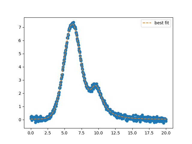
and figure:

plt.plot(x, data, 'o')
plt.plot(x, best_fit, '--', label='best fit')
plt.legend()
plt.show()