Using an ExpressionModel

ExpressionModels allow a model to be built from a user-supplied expression. See: https://lmfit.github.io/lmfit-py/builtin_models.html#user-defined-models

import matplotlib.pyplot as plt
import numpy as np

from lmfit.models import ExpressionModel

Generate synthetic data for the user-supplied model:

x = np.linspace(-10, 10, 201)
amp, cen, wid = 3.4, 1.8, 0.5

y = amp * np.exp(-(x-cen)**2 / (2*wid**2)) / (np.sqrt(2*np.pi)*wid)
np.random.seed(2021)
y = y + np.random.normal(size=x.size, scale=0.01)

Define the ExpressionModel and perform the fit:

gmod = ExpressionModel("amp * exp(-(x-cen)**2 /(2*wid**2))/(sqrt(2*pi)*wid)")
result = gmod.fit(y, x=x, amp=5, cen=5, wid=1)

this results in the following output:

print(result.fit_report())

[[Model]]
    <lmfit.ExpressionModel('amp * exp(-(x-cen)**2 /(2*wid**2))/(sqrt(2*pi)*wid)')>
[[Fit Statistics]]
    # fitting method   = leastsq
    # function evals   = 52
    # data points      = 201
    # variables        = 3
    chi-square         = 0.01951689
    reduced chi-square = 9.8570e-05
    Akaike info crit   = -1851.19580
    Bayesian info crit = -1841.28588
    R-squared          = 0.99967271
[[Variables]]
    amp:  3.40625133 +/- 0.00512077 (0.15%) (init = 5)
    cen:  1.80121155 +/- 8.6847e-04 (0.05%) (init = 5)
    wid:  0.50029616 +/- 8.6848e-04 (0.17%) (init = 1)
[[Correlations]] (unreported correlations are < 0.100)
    C(amp, wid) = +0.5774

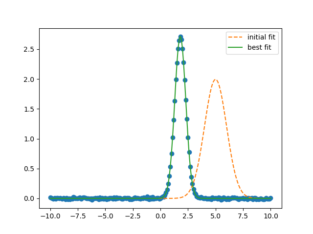
plt.plot(x, y, 'o')
plt.plot(x, result.init_fit, '--', label='initial fit')
plt.plot(x, result.best_fit, '-', label='best fit')
plt.legend()