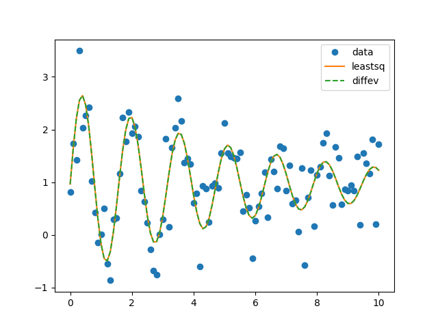
Fit Using differential_evolution Algorithm

This example compares the leastsq and differential_evolution algorithms on a fairly simple problem.

import matplotlib.pyplot as plt
import numpy as np

import lmfit


def resid(params, x, ydata):
    decay = params['decay'].value
    offset = params['offset'].value
    omega = params['omega'].value
    amp = params['amp'].value

    y_model = offset + amp * np.sin(x*omega) * np.exp(-x/decay)
    return y_model - ydata

Generate synthetic data and set-up Parameters with initial values/boundaries:

decay = 5
offset = 1.0
amp = 2.0
omega = 4.0

np.random.seed(2)
x = np.linspace(0, 10, 101)
y = offset + amp*np.sin(omega*x) * np.exp(-x/decay)
yn = y + np.random.normal(size=y.size, scale=0.450)

params = lmfit.Parameters()
params.add('offset', 2.0, min=0, max=10.0)
params.add('omega', 3.3, min=0, max=10.0)
params.add('amp', 2.5, min=0, max=10.0)
params.add('decay', 1.0, min=0, max=10.0)

Perform the fits and show fitting results and plot:

o1 = lmfit.minimize(resid, params, args=(x, yn), method='leastsq')
print("# Fit using leastsq:")
lmfit.report_fit(o1)

# Fit using leastsq:
[[Fit Statistics]]
    # fitting method   = leastsq
    # function evals   = 65
    # data points      = 101
    # variables        = 4
    chi-square         = 21.7961792
    reduced chi-square = 0.22470288
    Akaike info crit   = -146.871969
    Bayesian info crit = -136.411487
[[Variables]]
    offset:  0.96333089 +/- 0.04735890 (4.92%) (init = 2)
    omega:   3.98700839 +/- 0.02079709 (0.52%) (init = 3.3)
    amp:     1.80253587 +/- 0.19401928 (10.76%) (init = 2.5)
    decay:   5.76279753 +/- 1.04073348 (18.06%) (init = 1)
[[Correlations]] (unreported correlations are < 0.100)
    C(amp, decay) = -0.7550

o2 = lmfit.minimize(resid, params, args=(x, yn), method='differential_evolution')
print("\n\n# Fit using differential_evolution:")
lmfit.report_fit(o2)

# Fit using differential_evolution:
[[Fit Statistics]]
    # fitting method   = differential_evolution
    # function evals   = 1865
    # data points      = 101
    # variables        = 4
    chi-square         = 21.7961792
    reduced chi-square = 0.22470288
    Akaike info crit   = -146.871969
    Bayesian info crit = -136.411487
[[Variables]]
    offset:  0.96333018 +/- 0.04735904 (4.92%) (init = 2)
    omega:   3.98700832 +/- 0.02121808 (0.53%) (init = 3.3)
    amp:     1.80252738 +/- 0.19022472 (10.55%) (init = 2.5)
    decay:   5.76285571 +/- 1.00453329 (17.43%) (init = 1)
[[Correlations]] (unreported correlations are < 0.100)
    C(amp, decay) = -0.7434

plt.plot(x, yn, 'o', label='data')
plt.plot(x, yn+o1.residual, '-', label='leastsq')
plt.plot(x, yn+o2.residual, '--', label='diffev')
plt.legend()