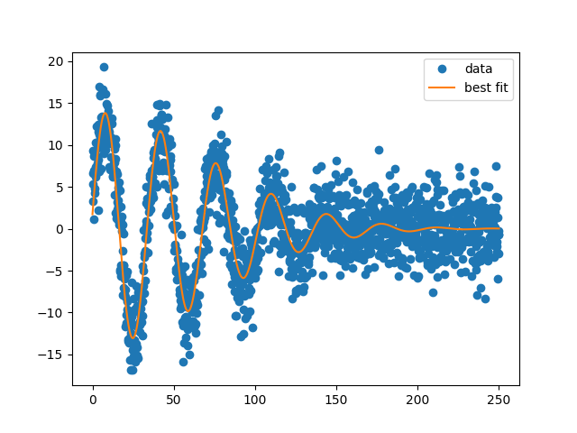
Fit Using Bounds

A major advantage of using lmfit is that one can specify boundaries on fitting parameters, even if the underlying algorithm in SciPy does not support this. For more information on how this is implemented, please refer to: https://lmfit.github.io/lmfit-py/bounds.html

The example below shows how to set boundaries using the min and max attributes to fitting parameters.

import matplotlib.pyplot as plt
from numpy import exp, linspace, pi, random, sign, sin

from lmfit import create_params, minimize
from lmfit.printfuncs import report_fit

create the ‘true’ Parameter values and residual function:

p_true = create_params(amp=14.0, period=5.4321, shift=0.12345, decay=0.010)


def residual(pars, x, data=None):
    argu = (x * pars['decay'])**2
    shift = pars['shift']
    if abs(shift) > pi/2:
        shift = shift - sign(shift)*pi
    model = pars['amp'] * sin(shift + x/pars['period']) * exp(-argu)
    if data is None:
        return model
    return model - data

Generate synthetic data and initialize fitting Parameters:

random.seed(0)
x = linspace(0, 250, 1500)
noise = random.normal(scale=2.8, size=x.size)
data = residual(p_true, x) + noise

fit_params = create_params(amp=dict(value=13, max=20, min=0),
                           period=dict(value=2, max=10),
                           shift=dict(value=0, max=pi/2., min=-pi/2.),
                           decay=dict(value=0.02, max=0.1, min=0))

Perform the fit and show the results:

out = minimize(residual, fit_params, args=(x,), kws={'data': data})
fit = residual(out.params, x)

report_fit(out, modelpars=p_true, correl_mode='table')

[[Fit Statistics]]
    # fitting method   = leastsq
    # function evals   = 79
    # data points      = 1500
    # variables        = 4
    chi-square         = 11301.3646
    reduced chi-square = 7.55438813
    Akaike info crit   = 3037.18756
    Bayesian info crit = 3058.44044
[[Variables]]
    amp:     13.8904759 +/- 0.24410753 (1.76%) (init = 13), model_value = 14
    period:  5.44026387 +/- 0.01416106 (0.26%) (init = 2), model_value = 5.4321
    shift:   0.12464389 +/- 0.02414210 (19.37%) (init = 0), model_value = 0.12345
    decay:   0.00996363 +/- 2.0275e-04 (2.03%) (init = 0.02), model_value = 0.01
[[Correlations]]
  +----------+----------+----------+----------+----------+
  | Variable | amp      | period   | shift    | decay    |
  +----------+----------+----------+----------+----------+
  | amp      | +1.0000  | -0.0700  | -0.0870  | +0.5757  |
  | period   | -0.0700  | +1.0000  | +0.7999  | -0.0404  |
  | shift    | -0.0870  | +0.7999  | +1.0000  | -0.0502  |
  | decay    | +0.5757  | -0.0404  | -0.0502  | +1.0000  |
  +----------+----------+----------+----------+----------+

plt.plot(x, data, 'o', label='data')
plt.plot(x, fit, label='best fit')
plt.legend()
plt.show()