Fit Specifying a Function to Compute the Jacobian

Specifying an analytical function to calculate the Jacobian can speed-up the fitting procedure.

import matplotlib.pyplot as plt
import numpy as np

from lmfit import Minimizer, Parameters


def func(pars, x, data=None):
    a, b, c = pars['a'], pars['b'], pars['c']
    model = a * np.exp(-b*x) + c
    if data is None:
        return model
    return model - data


def dfunc(pars, x, data=None):
    a, b = pars['a'], pars['b']
    v = np.exp(-b*x)
    return np.array([v, -a*x*v, np.ones(len(x))])


def f(var, x):
    return var[0] * np.exp(-var[1]*x) + var[2]


params = Parameters()
params.add('a', value=10)
params.add('b', value=10)
params.add('c', value=10)

a, b, c = 2.5, 1.3, 0.8
x = np.linspace(0, 4, 50)
y = f([a, b, c], x)
np.random.seed(2021)
data = y + 0.15*np.random.normal(size=x.size)

Fit without analytic derivative:

min1 = Minimizer(func, params, fcn_args=(x,), fcn_kws={'data': data})
out1 = min1.leastsq()
fit1 = func(out1.params, x)

Fit with analytic derivative:

min2 = Minimizer(func, params, fcn_args=(x,), fcn_kws={'data': data})
out2 = min2.leastsq(Dfun=dfunc, col_deriv=1)
fit2 = func(out2.params, x)

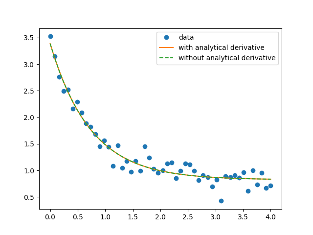
Comparison of fit to exponential decay with/without analytical derivatives to model = a*exp(-b*x) + c:

print(f'"true" parameters are: a = {a:.3f}, b = {b:.3f}, c = {c:.3f}\n\n'
      '|=========================================\n'
      '| Statistic/Parameter | Without | With   |\n'
      '|-----------------------------------------\n'
      f'|  N Function Calls   | {out1.nfev:d}      | {out2.nfev:d}     |\n'
      f'|     Chi-square      | {out1.chisqr:.4f}  | {out2.chisqr:.4f} |\n'
      f"|         a           | {out1.params['a'].value:.4f}  | {out2.params['a'].value:.4f} |\n"
      f"|         b           | {out1.params['b'].value:.4f}  | {out2.params['b'].value:.4f} |\n"
      f"|         c           | {out1.params['c'].value:.4f}  | {out2.params['c'].value:.4f} |\n"
      '------------------------------------------')

"true" parameters are: a = 2.500, b = 1.300, c = 0.800

|=========================================
| Statistic/Parameter | Without | With   |
|-----------------------------------------
|  N Function Calls   | 39      | 12     |
|     Chi-square      | 1.0920  | 1.0920 |
|         a           | 2.5635  | 2.5635 |
|         b           | 1.3585  | 1.3585 |
|         c           | 0.8241  | 0.8241 |
------------------------------------------

and the best-fit to the synthetic data (with added noise) is the same for both methods:

plt.plot(x, data, 'o', label='data')
plt.plot(x, fit1, label='with analytical derivative')
plt.plot(x, fit2, '--', label='without analytical derivative')
plt.legend()