Fit using the Model interface

This notebook shows a simple example of using the lmfit.Model class. For more information please refer to: https://lmfit.github.io/lmfit-py/model.html#the-model-class.

import numpy as np
from pandas import Series

from lmfit import Model, Parameter, report_fit

The Model class is a flexible, concise curve fitter. I will illustrate fitting example data to an exponential decay.

def decay(t, N, tau):
    return N*np.exp(-t/tau)

The parameters are in no particular order. We’ll need some example data. I will use N=7 and tau=3, and add a little noise.

t = np.linspace(0, 5, num=1000)
np.random.seed(2021)
data = decay(t, 7, 3) + np.random.randn(t.size)

Simplest Usage

model = Model(decay, independent_vars=['t'])
result = model.fit(data, t=t, N=10, tau=1)

The Model infers the parameter names by inspecting the arguments of the function, decay. Then I passed the independent variable, t, and initial guesses for each parameter. A residual function is automatically defined, and a least-squared regression is performed.

We can immediately see the best-fit values:

print(result.values)

{'N': 7.146693193035321, 'tau': 2.8980289807074064}

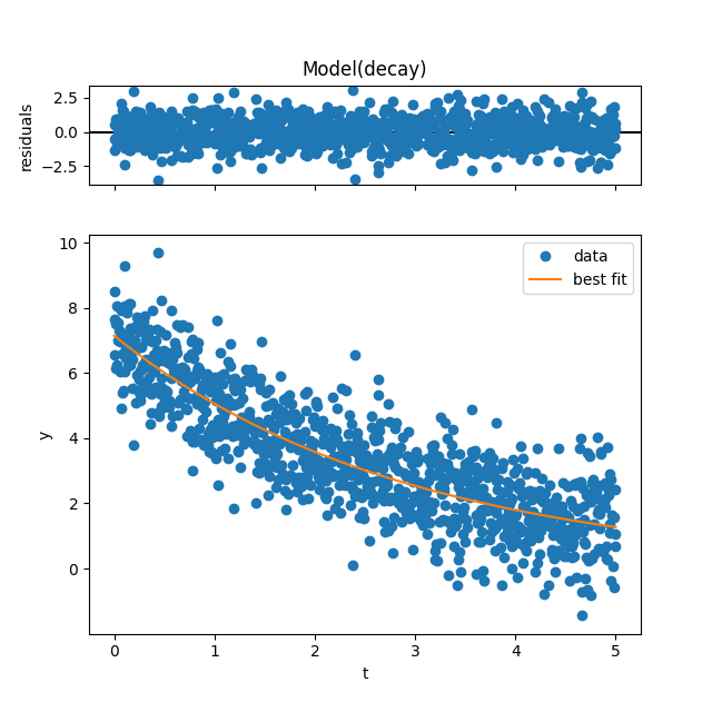
and use these best-fit parameters for plotting with the plot function:

result.plot()

We can review the best-fit Parameters by accessing result.params:

result.params.pretty_print()

Name     Value      Min      Max   Stderr     Vary     Expr Brute_Step
N       7.147     -inf      inf   0.0913     True     None     None
tau     2.898     -inf      inf  0.06299     True     None     None

More information about the fit is stored in the result, which is an lmfit.MimimizerResult object (see: https://lmfit.github.io/lmfit-py/fitting.html#lmfit.minimizer.MinimizerResult)

Specifying Bounds and Holding Parameters Constant

Above, the Model class implicitly builds Parameter objects from keyword arguments of fit that match the arguments of decay. You can build the Parameter objects explicitly; the following is equivalent.

result = model.fit(data, t=t,
                   N=Parameter('N', value=10),
                   tau=Parameter('tau', value=1))
report_fit(result.params)

[[Variables]]
    N:    7.14669319 +/- 0.09130428 (1.28%) (init = 10)
    tau:  2.89802898 +/- 0.06299118 (2.17%) (init = 1)
[[Correlations]] (unreported correlations are < 0.100)
    C(N, tau) = -0.7533

By building Parameter objects explicitly, you can specify bounds (min, max) and set parameters constant (vary=False).

result = model.fit(data, t=t,
                   N=Parameter('N', value=7, vary=False),
                   tau=Parameter('tau', value=1, min=0))
report_fit(result.params)

[[Variables]]
    N:    7 (fixed)
    tau:  2.97663118 +/- 0.04347476 (1.46%) (init = 1)

Defining Parameters in Advance

Passing parameters to fit can become unwieldy. As an alternative, you can extract the parameters from model like so, set them individually, and pass them to fit.

params = model.make_params(N=10, tau={'value': 1, 'min': 0})

result = model.fit(data, params, t=t)
report_fit(result.params)

[[Variables]]
    N:    7.14669316 +/- 0.09130423 (1.28%) (init = 10)
    tau:  2.89802901 +/- 0.06299127 (2.17%) (init = 1)
[[Correlations]] (unreported correlations are < 0.100)
    C(N, tau) = -0.7533

Keyword arguments override params, resetting value and all other properties (min, max, vary).

result = model.fit(data, params, t=t, tau=1)
report_fit(result.params)

[[Variables]]
    N:    7.14669316 +/- 0.09130423 (1.28%) (init = 10)
    tau:  2.89802901 +/- 0.06299127 (2.17%) (init = 1)
[[Correlations]] (unreported correlations are < 0.100)
    C(N, tau) = -0.7533

The input parameters are not modified by fit. They can be reused, retaining the same initial value. If you want to use the result of one fit as the initial guess for the next, simply pass params=result.params.

#TODO/FIXME: not sure if there ever way a “helpful exception”, but currently #it raises a ValueError: The input contains nan values.

#*A Helpful Exception*

#All this implicit magic makes it very easy for the user to neglect to set a #parameter. The fit function checks for this and raises a helpful exception.

# #result = model.fit(data, t=t, tau=1)  # N unspecified

#An extra parameter that cannot be matched to the model function will #throw a UserWarning, but it will not raise, leaving open the possibility #of unforeseen extensions calling for some parameters.

Weighted Fits

Use the sigma argument to perform a weighted fit. If you prefer to think of the fit in term of weights, sigma=1/weights.

weights = np.arange(len(data))
result = model.fit(data, params, t=t, weights=weights)
report_fit(result.params)

[[Variables]]
    N:    6.98535179 +/- 0.28002384 (4.01%) (init = 10)
    tau:  2.97268236 +/- 0.11134755 (3.75%) (init = 1)
[[Correlations]] (unreported correlations are < 0.100)
    C(N, tau) = -0.9311

Handling Missing Data

By default, attempting to fit data that includes a NaN, which conventionally indicates a “missing” observation, raises a lengthy exception. You can choose to omit (i.e., skip over) missing values instead.

data_with_holes = data.copy()
data_with_holes[[5, 500, 700]] = np.nan  # Replace arbitrary values with NaN.

model = Model(decay, independent_vars=['t'], nan_policy='omit')
result = model.fit(data_with_holes, params, t=t)
report_fit(result.params)

[[Variables]]
    N:    7.15448795 +/- 0.09181809 (1.28%) (init = 10)
    tau:  2.89285089 +/- 0.06306004 (2.18%) (init = 1)
[[Correlations]] (unreported correlations are < 0.100)
    C(N, tau) = -0.7542

If you don’t want to ignore missing values, you can set the model to raise proactively, checking for missing values before attempting the fit.

Uncomment to see the error #model = Model(decay, independent_vars=[‘t’], nan_policy=’raise’) #result = model.fit(data_with_holes, params, t=t)

The default setting is nan_policy='raise', which does check for NaNs and raises an exception when present.

Null-checking relies on pandas.isnull if it is available. If pandas cannot be imported, it silently falls back on numpy.isnan.

Data Alignment

Imagine a collection of time series data with different lengths. It would be convenient to define one sufficiently long array t and use it for each time series, regardless of length. pandas (https://pandas.pydata.org/pandas-docs/stable/) provides tools for aligning indexed data. And, unlike most wrappers to scipy.leastsq, Model can handle pandas objects out of the box, using its data alignment features.

Here I take just a slice of the data and fit it to the full t. It is automatically aligned to the correct section of t using Series’ index.

model = Model(decay, independent_vars=['t'])
truncated_data = Series(data)[200:800]  # data points 200-800
t = Series(t)  # all 1000 points
result = model.fit(truncated_data, params, t=t)
report_fit(result.params)

[[Variables]]
    N:    7.10725864 +/- 0.24259071 (3.41%) (init = 10)
    tau:  2.92503564 +/- 0.13481789 (4.61%) (init = 1)
[[Correlations]] (unreported correlations are < 0.100)
    C(N, tau) = -0.9320

Data with missing entries and an unequal length still aligns properly.

model = Model(decay, independent_vars=['t'], nan_policy='omit')
truncated_data_with_holes = Series(data_with_holes)[200:800]
result = model.fit(truncated_data_with_holes, params, t=t)
report_fit(result.params)

[[Variables]]
    N:    7.11270194 +/- 0.24334895 (3.42%) (init = 10)
    tau:  2.92065227 +/- 0.13488230 (4.62%) (init = 1)
[[Correlations]] (unreported correlations are < 0.100)
    C(N, tau) = -0.9320