Fit Multiple Data Sets Using Model Interface

Fitting multiple (simulated) Gaussian data sets simultaneously, using the Model interface.

All minimizers require the residual array to be one-dimensional. Therefore, in the objective function we need to flatten the array before returning it.

import matplotlib.pyplot as plt
import numpy as np

from lmfit import Parameters, minimize, report_fit
from lmfit.models import GaussianModel

Create N simulated Gaussian data sets

N = 5
np.random.seed(2021)
x = np.linspace(-1, 2, 151)
data = []
for _ in np.arange(N):
    params = Parameters()
    params.add('amplitude', value=0.60 + 9.50*np.random.rand())
    params.add('center', value=-0.20 + 1.20*np.random.rand())
    params.add('sigma', value=0.25 + 0.03*np.random.rand())
    dat = (GaussianModel().eval(x=x, params=params) +
           np.random.normal(size=x.size, scale=0.1))
    data.append(dat)
data = np.array(data)

The objective function will extract and evaluate a Gaussian from the compound model

def objective(params, x, data, model):
    """Calculate total residual for fits of Gaussians to several data sets."""
    ndata, _ = data.shape
    resid = 0.0*data[:]

    # make residual per data set
    for i in range(ndata):
        components = model.components[i].eval(params=params, x=x)
        resid[i, :] = data[i, :] - components

    # now flatten this to a 1D array, as minimize() needs
    return resid.flatten()

Create a composite model by adding Gaussians

model_arr = [GaussianModel(prefix=f'n{i+1}_') for i, _ in enumerate(data)]
model = sum(model_arr[1:], start=model_arr[0])

Prepare the fitting parameters and constrain n2_sigma, …, nN_sigma to be equal to n1_sigma

fit_params = model.make_params()
for iy, y in enumerate(data):
    fit_params.add(f'n{iy+1}_amplitude', value=0.5, min=0.0, max=200)
    fit_params.add(f'n{iy+1}_center', value=0.4, min=-2.0, max=2.0)
    fit_params.add(f'n{iy+1}_sigma', value=0.3, min=0.01, max=3.0)

    if iy > 0:
        fit_params[f'n{iy+1}_sigma'].expr = 'n1_sigma'

Run the global fit and show the fitting result

out = minimize(objective, fit_params, args=(x, data, model))
report_fit(out.params)

[[Variables]]
    n1_amplitude:  6.40552155 +/- 0.01575090 (0.25%) (init = 0.5)
    n1_center:     0.68032886 +/- 8.6209e-04 (0.13%) (init = 0.4)
    n1_sigma:      0.25743367 +/- 3.4131e-04 (0.13%) (init = 0.3)
    n2_amplitude:  6.98975626 +/- 0.01585971 (0.23%) (init = 0.5)
    n2_center:     0.50446887 +/- 7.9004e-04 (0.16%) (init = 0.4)
    n2_sigma:      0.25743367 +/- 3.4131e-04 (0.13%) == 'n1_sigma'
    n3_amplitude:  7.30195609 +/- 0.01592142 (0.22%) (init = 0.5)
    n3_center:    -0.08261146 +/- 7.5626e-04 (0.92%) (init = 0.4)
    n3_sigma:      0.25743367 +/- 3.4131e-04 (0.13%) == 'n1_sigma'
    n4_amplitude:  6.01461340 +/- 0.01568302 (0.26%) (init = 0.5)
    n4_center:     0.07382999 +/- 9.1812e-04 (1.24%) (init = 0.4)
    n4_sigma:      0.25743367 +/- 3.4131e-04 (0.13%) == 'n1_sigma'
    n5_amplitude:  9.07744386 +/- 0.01631785 (0.18%) (init = 0.5)
    n5_center:     0.34402084 +/- 6.0834e-04 (0.18%) (init = 0.4)
    n5_sigma:      0.25743367 +/- 3.4131e-04 (0.13%) == 'n1_sigma'
    n1_fwhm:       0.60620995 +/- 8.0373e-04 (0.13%) == '2.3548200*n1_sigma'
    n1_height:     9.92657076 +/- 0.02440907 (0.25%) == '0.3989423*n1_amplitude/max(1e-15, n1_sigma)'
    n2_fwhm:       0.60620995 +/- 8.0373e-04 (0.13%) == '2.3548200*n2_sigma'
    n2_height:     10.8319533 +/- 0.02457770 (0.23%) == '0.3989423*n2_amplitude/max(1e-15, n2_sigma)'
    n3_fwhm:       0.60620995 +/- 8.0373e-04 (0.13%) == '2.3548200*n3_sigma'
    n3_height:     11.3157661 +/- 0.02467331 (0.22%) == '0.3989423*n3_amplitude/max(1e-15, n3_sigma)'
    n4_fwhm:       0.60620995 +/- 8.0373e-04 (0.13%) == '2.3548200*n4_sigma'
    n4_height:     9.32078443 +/- 0.02430386 (0.26%) == '0.3989423*n4_amplitude/max(1e-15, n4_sigma)'
    n5_fwhm:       0.60620995 +/- 8.0373e-04 (0.13%) == '2.3548200*n5_sigma'
    n5_height:     14.0672212 +/- 0.02528769 (0.18%) == '0.3989423*n5_amplitude/max(1e-15, n5_sigma)'
[[Correlations]] (unreported correlations are < 0.100)
    C(n1_sigma, n5_amplitude)     = +0.3688
    C(n1_sigma, n3_amplitude)     = +0.3040
    C(n1_sigma, n2_amplitude)     = +0.2922
    C(n1_amplitude, n1_sigma)     = +0.2696
    C(n1_sigma, n4_amplitude)     = +0.2542
    C(n3_amplitude, n5_amplitude) = +0.1121
    C(n2_amplitude, n5_amplitude) = +0.1077

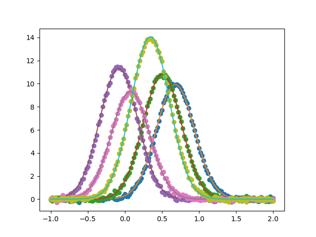
Plot the data sets and fits

plt.figure()
for i, y in enumerate(data):
    components = model.eval_components(params=out.params, x=x)
    plt.plot(x, y, 'o', x, components[f'n{i+1}_'], '-')

plt.show()