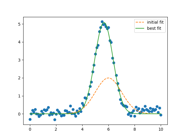
doc_model_with_nan_policy.py

[[Model]]
    Model(gaussian)
[[Fit Statistics]]
    # fitting method   = leastsq
    # function evals   = 22
    # data points      = 99
    # variables        = 3
    chi-square         = 3.27990355
    reduced chi-square = 0.03416566
    Akaike info crit   = -331.323278
    Bayesian info crit = -323.537918
    R-squared          = 0.98570688
[[Variables]]
    amplitude:  8.82064881 +/- 0.11686114 (1.32%) (init = 5)
    center:     5.65906365 +/- 0.01055590 (0.19%) (init = 6)
    sigma:      0.69165307 +/- 0.01060640 (1.53%) (init = 1)
    fwhm:       1.62871849 +/- 0.02497615 (1.53%) == '2.3548200*sigma'
    height:     5.08770952 +/- 0.06488251 (1.28%) == '0.3989423*amplitude/max(1e-15, sigma)'
[[Correlations]] (unreported correlations are < 0.100)
    C(amplitude, sigma) = +0.6105

# <examples/doc_model_with_nan_policy.py>
import matplotlib.pyplot as plt
import numpy as np

from lmfit.models import GaussianModel

data = np.loadtxt('model1d_gauss.dat')
x = data[:, 0]
y = data[:, 1]

y[44] = np.nan
y[65] = np.nan

# nan_policy = 'raise'
# nan_policy = 'propagate'
nan_policy = 'omit'

gmodel = GaussianModel()
result = gmodel.fit(y, x=x, amplitude=5, center=6, sigma=1,
                    nan_policy=nan_policy)

print(result.fit_report())

# make sure nans are removed for plotting:
x_ = x[np.where(np.isfinite(y))]
y_ = y[np.where(np.isfinite(y))]

plt.plot(x_, y_, 'o')
plt.plot(x_, result.init_fit, '--', label='initial fit')
plt.plot(x_, result.best_fit, '-', label='best fit')
plt.legend()
plt.show()
# <end examples/doc_model_with_nan_policy.py>