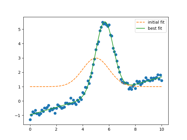
doc_model_two_components.py

[[Model]]
    (Model(gaussian) + Model(line))
[[Fit Statistics]]
    # fitting method   = leastsq
    # function evals   = 55
    # data points      = 101
    # variables        = 5
    chi-square         = 2.57855517
    reduced chi-square = 0.02685995
    Akaike info crit   = -360.457020
    Bayesian info crit = -347.381417
    R-squared          = 0.99194643
[[Variables]]
    amp:        8.45930976 +/- 0.12414531 (1.47%) (init = 5)
    cen:        5.65547889 +/- 0.00917673 (0.16%) (init = 5)
    wid:        0.67545513 +/- 0.00991697 (1.47%) (init = 1)
    slope:      0.26484403 +/- 0.00574892 (2.17%) (init = 0)
    intercept: -0.96860189 +/- 0.03352202 (3.46%) (init = 1)
[[Correlations]] (unreported correlations are < 0.100)
    C(slope, intercept) = -0.7954
    C(amp, wid)         = +0.6664
    C(amp, intercept)   = -0.2216
    C(amp, slope)       = -0.1692
    C(cen, slope)       = -0.1618
    C(wid, intercept)   = -0.1477
    C(cen, intercept)   = +0.1287
    C(wid, slope)       = -0.1127

# <examples/doc_model_two_components.py>
import matplotlib.pyplot as plt
from numpy import exp, loadtxt, pi, sqrt

from lmfit import Model

data = loadtxt('model1d_gauss.dat')
x = data[:, 0]
y = data[:, 1] + 0.25*x - 1.0


def gaussian(x, amp, cen, wid):
    """1-d gaussian: gaussian(x, amp, cen, wid)"""
    return (amp / (sqrt(2*pi) * wid)) * exp(-(x-cen)**2 / (2*wid**2))


def line(x, slope, intercept):
    """a line"""
    return slope*x + intercept


mod = Model(gaussian) + Model(line)
pars = mod.make_params(amp=5, cen=5, wid={'value': 1, 'min': 0},
                       slope=0, intercept=1)

result = mod.fit(y, pars, x=x)
print(result.fit_report())

plt.plot(x, y, 'o')
plt.plot(x, result.init_fit, '--', label='initial fit')
plt.plot(x, result.best_fit, '-', label='best fit')
plt.legend()
plt.show()
# <end examples/doc_model_two_components.py>