Calculate Confidence Intervals

import matplotlib.pyplot as plt
from numpy import argsort, exp, linspace, pi, random, sign, sin, unique
from scipy.interpolate import interp1d

from lmfit import (Minimizer, conf_interval, conf_interval2d, create_params,
                   report_ci, report_fit)

Define the residual function, specify “true” parameter values, and generate a synthetic data set with some noise:

def residual(pars, x, data=None):
    argu = (x*pars['decay'])**2
    shift = pars['shift']
    if abs(shift) > pi/2:
        shift = shift - sign(shift)*pi
    model = pars['amp']*sin(shift + x/pars['period']) * exp(-argu)
    if data is None:
        return model
    return model - data


p_true = create_params(amp=14.0, period=5.33, shift=0.123, decay=0.010)

x = linspace(0.0, 250.0, 2500)
random.seed(2021)
noise = random.normal(scale=0.7215, size=x.size)
data = residual(p_true, x) + noise

Create fitting parameters and set initial values:

fit_params = create_params(amp=13.0, period=2, shift=0.0, decay=0.020)

Set-up the minimizer and perform the fit using leastsq algorithm, and show the report:

mini = Minimizer(residual, fit_params, fcn_args=(x,), fcn_kws={'data': data})
out = mini.leastsq()

fit = residual(out.params, x)
report_fit(out)

[[Fit Statistics]]
    # fitting method   = leastsq
    # function evals   = 95
    # data points      = 2500
    # variables        = 4
    chi-square         = 1277.24638
    reduced chi-square = 0.51171730
    Akaike info crit   = -1670.96059
    Bayesian info crit = -1647.66441
[[Variables]]
    amp:     14.0708269 +/- 0.04936878 (0.35%) (init = 13)
    period:  5.32980958 +/- 0.00273143 (0.05%) (init = 2)
    shift:   0.12156317 +/- 0.00482312 (3.97%) (init = 0)
    decay:   0.01002489 +/- 4.0726e-05 (0.41%) (init = 0.02)
[[Correlations]] (unreported correlations are < 0.100)
    C(period, shift) = +0.8002
    C(amp, decay)    = +0.5758

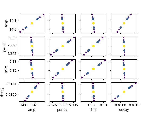
Calculate the confidence intervals for parameters and display the results:

ci, tr = conf_interval(mini, out, trace=True)

report_ci(ci)

names = out.params.keys()
i = 0
gs = plt.GridSpec(4, 4)
sx = {}
sy = {}
for fixed in names:
    j = 0
    for free in names:
        if j in sx and i in sy:
            ax = plt.subplot(gs[i, j], sharex=sx[j], sharey=sy[i])
        elif i in sy:
            ax = plt.subplot(gs[i, j], sharey=sy[i])
            sx[j] = ax
        elif j in sx:
            ax = plt.subplot(gs[i, j], sharex=sx[j])
            sy[i] = ax
        else:
            ax = plt.subplot(gs[i, j])
            sy[i] = ax
            sx[j] = ax
        if i < 3:
            plt.setp(ax.get_xticklabels(), visible=False)
        else:
            ax.set_xlabel(free)

        if j > 0:
            plt.setp(ax.get_yticklabels(), visible=False)
        else:
            ax.set_ylabel(fixed)

        res = tr[fixed]
        prob = res['prob']
        f = prob < 0.96

        x, y = res[free], res[fixed]
        ax.scatter(x[f], y[f], c=1-prob[f], s=25*(1-prob[f]+0.5))
        ax.autoscale(1, 1)
        j += 1
    i += 1

          99.73%    95.45%    68.27%    _BEST_    68.27%    95.45%    99.73%
amp   :  -0.14795  -0.09863  -0.04934  14.07083  +0.04939  +0.09886  +0.14847
period:  -0.00818  -0.00546  -0.00273   5.32981  +0.00273  +0.00548  +0.00822
shift :  -0.01446  -0.00964  -0.00482   0.12156  +0.00482  +0.00965  +0.01449
decay :  -0.00012  -0.00008  -0.00004   0.01002  +0.00004  +0.00008  +0.00012

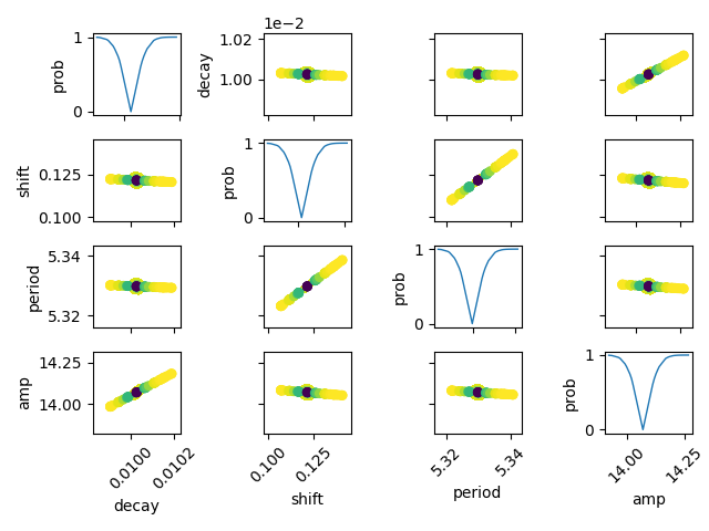
It is also possible to calculate the confidence regions for two fixed parameters using the function conf_interval2d:

names = list(out.params.keys())

plt.figure()
for i in range(4):
    for j in range(4):
        indx = 16-j*4-i
        ax = plt.subplot(4, 4, indx)
        ax.ticklabel_format(style='sci', scilimits=(-2, 2), axis='y')

        # set-up labels and tick marks
        ax.tick_params(labelleft=False, labelbottom=False)
        if indx in (2, 5, 9, 13):
            plt.ylabel(names[j])
            ax.tick_params(labelleft=True)
        if indx == 1:
            ax.tick_params(labelleft=True)
        if indx in (13, 14, 15, 16):
            plt.xlabel(names[i])
            ax.tick_params(labelbottom=True)
            [label.set_rotation(45) for label in ax.get_xticklabels()]

        if i != j:
            x, y, m = conf_interval2d(mini, out, names[i], names[j], 20, 20)
            plt.contourf(x, y, m, linspace(0, 1, 10))

            x = tr[names[i]][names[i]]
            y = tr[names[i]][names[j]]
            pr = tr[names[i]]['prob']
            s = argsort(x)
            plt.scatter(x[s], y[s], c=pr[s], s=30, lw=1)

        else:
            x = tr[names[i]][names[i]]
            y = tr[names[i]]['prob']

            t, s = unique(x, True)
            f = interp1d(t, y[s], 'slinear')
            xn = linspace(x.min(), x.max(), 50)
            plt.plot(xn, f(xn), lw=1)
            plt.ylabel('prob')
            ax.tick_params(labelleft=True)

plt.tight_layout()
plt.show()